Example Usage¶

import sgmdata
import pandas
import numpy as np
from matplotlib import pyplot as plt 

Loading BokehJS ...

Dask Background¶

The whole sgm-data library makes use ‘dask’ arrays, this allows for multiprocessing capabilities, in a ‘pandas-like’ programming environment. The dask client is useful for very large datasets, it sets up workers to propogate your data and the operations upon it across several worker processes / nodes. For more about dask visit their website

The below cell is optional and, if run, should only be run once per session. Dask will work quicker on small operations without the client (but you may run out of memory).

from dask.distributed import Client
client = Client('dscheduler:8786') ## Can also run Client() for smaller jobs (could be faster).

Searching for Data¶

You can find your data in the SGMLive database by using the SGMQuery module. The following documentation details the keywords that you can use to customize your search.

class SGMQuery(**kwargs):¶

sample (str:required) At minimum you’ll need to provide the keyword “sample”, corresponding the sample name in the database as a default this will grab all the data under that sample name.

daterange (tuple:optional) This can be used to sort through sample data by the day that it was acquired. This is designed to take a tuple of the form ("start-date", "end-date") where the strings are of the form "YYYY-MM-DD". You can also just use a single string of the same form, instead of a tuple, this will make the assumption that “end-date” == now().

data (bool:optional) As a default (True) the SGMQuery object will try to load the the data from disk, if this is not the desired behaviour set data=False.

user (str:optional:staffonly) Can be used to select the username in SGMLive from which the sample query is performed. Not available to non-staff.

processed (bool:optional) Can be used to return the paths for the processed data (already interpolated) instead of the raw. You would generally set data = False for this option.

Attributes¶

data (object) By default the query will create an SGMData object containing your data, this can be turned off with the data keyword.

paths (list). Contains the local paths to your data (or processed_data if processed=True).

%%time
sgmq = sgmdata.SGMQuery(sample="TeCN - C", user='arthurz')

sgm_data = sgmq.data

Loading Data¶

Data can be loaded in as a single file path, or as a list or paths. The actual data is only loaded as a representation at first. By default SGMQuery creates an SGMData object under the property ‘data’.

class SGMData(file_paths, **kwargs):¶

arg¶

Keywords¶

axes (str:optional) At minimum you’ll need to provide the keyword “sample”, corresponding the sample name in the database as a default this will grab all the data under that sample name.

daterange (tuple:optional) This can be used to sort through sample data by the day that it was acquired. This is designed to take a tuple of the form ("start-date", "end-date") where the strings are of the form "YYYY-MM-DD". You can also just use a single string of the same form, instead of a tuple, this will make the assumption that “end-date” == now().

data (bool:optional) As a default (True) the SGMQuery object will try to load the the data from disk, if this is not the desired behaviour set data=False.

user (str:optional:staffonly) Can be used to select the username in SGMLive from which the sample query is performed. Not available to non-staff.

processed (bool:optional) Can be used to return the paths for the processed data (already interpolated) instead of the raw. You would generally set data = False for this option.

Functions¶

Attributes¶

scans (object) By default the query will create an SGMData object containing your data, this can be turned off with the data keyword.

paths (list). Contains the local paths to your data (or processed_data if processed=True).

The data is auto grouped into three classifications: “independent”, “signals”, and “other”. You can view the data dictionary representation in a Jupyter cell by just invoking the SGMData() object.

from sgmdata import preprocess
preprocess(sample="TeCN - C", user='arthurz', resolution=0.1, client=client)

Averaged 10 scans for TeCN - C

The SGMScan object¶

Contains a representation in memory of the data loaded from disk, plus any interpolated scans.

sgm_data.scans['2022-02-08t14-56-25-0600']

	Sample	Command	Independent	Signals	Other
entry3	TeCN - C	['cscan', 'en', '270', '320', '60']	['en']	['aux1', 'clock', 'i0', 'pd', 'sdd1', 'sdd2', 'sdd3', 'sdd4', 'temp1', 'temp2', 'tey']	['emission', 'image']

sgm_data.scans['2021-08-18t04-14-47-0600'].entry1.command

['eemscan', 'en', '270', '2000', '60', '100']

sgm_data.scans['2021-08-18t04-14-47-0600'].entry1.independent['en']

	Array	Chunk
Bytes	137.20 kiB	45.73 kiB
Shape	(35123,)	(11707,)
Count	5 Tasks	4 Chunks
Type	float32	numpy.ndarray

35123 1

sgm_data.scans['2021-08-18t04-14-47-0600'].entry1.signals['tey']

	Array	Chunk
Bytes	137.20 kiB	45.73 kiB
Shape	(35123,)	(11707,)
Count	5 Tasks	4 Chunks
Type	float32	numpy.ndarray

35123 1

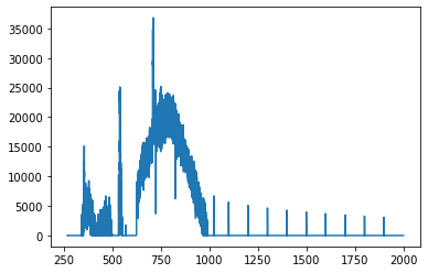
Plotting Scan Data¶

For individual plots, you can visualize access the data, and plot it manually, or you can use the plot() routine. If interpolation step has already been performed, the data will be from that source.

en = sgm_data.scans['2021-08-18t04-14-47-0600'].entry1.independent['en']
tey = sgm_data.scans['2021-08-18t04-14-47-0600'].entry1.signals['tey']

plt.plot(en,tey)

[<matplotlib.lines.Line2D at 0x7f3fad40ffd0>]

png

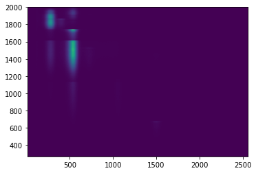
arr = sgm_data.scans['2021-08-18t04-14-47-0600'].entry1.signals['sdd3']
plt.imshow(arr, extent=[10,2560, 270, 2000])

<matplotlib.image.AxesImage at 0x7f3fad319550>

png

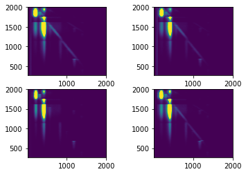
arr1 = sgm_data.scans['2021-08-18t04-14-47-0600'].entry1.signals['sdd1']
arr2 = sgm_data.scans['2021-08-18t04-14-47-0600'].entry1.signals['sdd2']
arr3 = sgm_data.scans['2021-08-18t04-14-47-0600'].entry1.signals['sdd3']
arr4 = sgm_data.scans['2021-08-18t04-14-47-0600'].entry1.signals['sdd4']

fig, axs = plt.subplots(2, 2)
axs[0,0].imshow(arr1, extent=[10,2000, 270, 2000], vmin = 1, vmax = 1000)
axs[0,1].imshow(arr2, extent=[10,2000, 270, 2000], vmin = 1, vmax = 1000)
axs[1,0].imshow(arr3, extent=[10,2000, 270, 2000], vmin = 1, vmax = 1000)
axs[1,1].imshow(arr4, extent=[10,2000, 270, 2000], vmin = 1, vmax = 1000)

<matplotlib.image.AxesImage at 0x7f3f8c2b25b0>

png

sgm_data.scans['2021-08-18t04-14-47-0600'].entry1.plot()

Interpolating Data¶

Individual scans are loaded into the SGMData namespace, and can be interpolated from here. By selecting compute == False we can stage the dask array computation to occur at a later time (e.g. by running object.compute()).

df = sgm_data.scans['2021-08-18t04-14-47-0600'].entry1.interpolate(resolution=0.25)

sgm_data.scans['2021-01-21t13-47-04-0600'].entry2.keys()

dict_keys(['command', 'sample', 'description', 'independent', 'signals', 'other', 'npartitions', 'new_axes', 'dataframe', 'binned'])

sgm_data.scans['2021-01-21t13-47-04-0600'].entry2.binned['dataframe']

	aux1	clock	i0	pd	sdd1-0	sdd1-1	sdd1-2	sdd1-3	sdd1-4	sdd1-5	...	sdd4-249	sdd4-250	sdd4-251	sdd4-252	sdd4-253	sdd4-254	sdd4-255	temp1	temp2	tey
en
440.000000	0.0	0.022239	72052.909091	403.454545	0.0	0.0	0.0	0.0	0.0	0.0	...	0.0	0.0	0.0	0.0	0.0	0.0	0.0	81.363636	186.818182	12242.818182
440.100167	0.0	0.022102	69012.800000	415.800000	0.0	0.0	0.0	0.0	0.0	0.0	...	0.0	0.0	0.0	0.0	0.0	0.0	0.0	72.000000	181.200000	12866.400000
440.200334	0.0	0.022747	73289.000000	402.714286	0.0	0.0	0.0	0.0	0.0	0.0	...	0.0	0.0	0.0	0.0	0.0	0.0	0.0	79.857143	193.428571	12280.000000
440.300501	0.0	0.022295	71447.500000	411.000000	0.0	0.0	0.0	0.0	0.0	0.0	...	0.0	0.0	0.0	0.0	0.0	0.0	0.0	81.333333	187.166667	12558.166667
440.400668	0.0	0.022429	71883.166667	408.333333	0.0	0.0	0.0	0.0	0.0	0.0	...	0.0	0.0	0.0	0.0	0.0	0.0	0.0	81.166667	192.833333	12588.000000
...	...	...	...	...	...	...	...	...	...	...	...	...	...	...	...	...	...	...	...	...	...
499.599332	0.0	0.019963	83576.600000	390.200000	0.0	0.0	0.0	0.0	0.0	0.0	...	0.0	0.0	0.0	0.0	0.0	0.0	0.0	79.800000	179.800000	36676.000000
499.699499	0.0	0.020021	85236.166667	391.000000	0.0	0.0	0.0	0.0	0.0	0.0	...	0.0	0.0	0.0	0.0	0.0	0.0	0.0	90.333333	190.666667	36227.333333
499.799666	0.0	0.019952	84377.800000	400.600000	0.0	0.0	0.0	0.0	0.0	0.0	...	0.0	0.0	0.0	0.0	0.0	0.0	0.0	79.600000	190.200000	36549.800000
499.899833	0.0	0.019913	82349.000000	393.000000	0.0	0.0	0.0	0.0	0.0	0.0	...	0.0	0.0	0.0	0.0	0.0	0.0	0.0	74.666667	183.500000	36853.833333
500.000000	0.0	0.021838	84041.473214	392.348214	0.0	0.0	0.0	0.0	0.0	0.0	...	0.0	0.0	0.0	0.0	0.0	0.0	0.0	80.339286	188.361607	36589.477679

600 rows × 1031 columns

sgm_data.scans['2021-01-21t13-47-04-0600'].entry2.plot()

Plotting Interpolated Data

Batch interpolation¶

You can also batch interpolate the loaded scans from the top of the namespace.
Note: this process is only applicable if all scans loaded in the namespace can take the same interpolation parameters.

%%time
interp_list = sgm_data.interpolate(resolution=0.1, start=450, stop=470)

  0%|          | 0/10 [00:00<?, ?it/s]


CPU times: user 27.3 s, sys: 15.1 s, total: 42.4 s
Wall time: 42.2 s

Averaging Data¶

Scans that are loaded into the SGMData namespace, with a corresponding sample name and command can be grouped together and averaged.

%%time
averaged = sgm_data.mean()

CPU times: user 49 ms, sys: 26.7 ms, total: 75.7 ms
Wall time: 56.5 ms

You can plot Averaged Data, from the list of ‘like’ scans using the plot() function.

sgm_data.averaged['TiO2 - Ti'][0].plot()

df =averaged['TiO2 - Ti'][0]['data']

df.filter(regex="sdd2.*").to_numpy().shape

(200, 256)

Fitting XRF Spectra¶

Using any data set for which an interpolation has already been performed, the fit_mcas function can be used to find peaks and batch fit them for all four sdd detectors.

%%time
sgm_data = sgmdata.SGMQuery(sample="Focus Testing 2").data
sgm_data

  0%|          | 0/35 [00:00<?, ?it/s]

CPU times: user 2.63 s, sys: 784 ms, total: 3.41 s
Wall time: 5.07 s

/opt/conda/lib/python3.8/site-packages/sgmdata/load.py:493: UserWarning: Some scan files were not loaded: ['2021-07-29t14-49-46-0600', '2021-07-29t11-24-27-0600']
  warnings.warn(f"Some scan files were not loaded: {err}")

File	Entry	Sample	Command	Independent	Signals	Other
2021-07-29t14-54-37-0600	entry35	Focus Testing 2	['cmesh', 'xp', '6.2', '5.7', '10', 'yp', '-0.8', '-1.1']	['xp', 'yp']	['aux1', 'clock', 'i0', 'pd', 'sdd1', 'sdd2', 'sdd3', 'sdd4', 'temp1', 'temp2', 'tey']	['emission', 'image']
2021-07-29t14-46-01-0600	entry33	Focus Testing 2	['cscan', 'hex_y', '-9.5576', '-8.5576']	['hex_y']	['aux1', 'clock', 'i0', 'pd', 'sdd1', 'sdd2', 'sdd3', 'sdd4', 'temp1', 'temp2', 'tey']	['emission', 'image']
2021-07-29t14-45-30-0600	entry32	Focus Testing 2	['cscan', 'hex_x', '-2.1949', '-1.1949']	['hex_x']	['aux1', 'clock', 'i0', 'pd', 'sdd1', 'sdd2', 'sdd3', 'sdd4', 'temp1', 'temp2', 'tey']	['emission', 'image']
2021-07-29t14-30-48-0600	entry31	Focus Testing 2	['cscan', 'hex_y', '-9.5576', '-8.5576']	['hex_y']	['aux1', 'clock', 'i0', 'pd', 'sdd1', 'sdd2', 'sdd3', 'sdd4', 'temp1', 'temp2', 'tey']	['emission', 'image']
2021-07-29t14-27-43-0600	entry30	Focus Testing 2	['cscan', 'hex_x', '-2.1949', '-1.1949']	['hex_x']	['aux1', 'clock', 'i0', 'pd', 'sdd1', 'sdd2', 'sdd3', 'sdd4', 'temp1', 'temp2', 'tey']	['emission', 'image']
2021-07-29t13-04-30-0600	entry29	Focus Testing 2	['cmesh', 'xp', '7', '5', '10', 'yp', '1', '-1']	['xp', 'yp']	['aux1', 'clock', 'i0', 'pd', 'sdd1', 'sdd2', 'sdd3', 'sdd4', 'temp1', 'temp2', 'tey']	['emission', 'image']
2021-07-29t13-01-16-0600	entry28	Focus Testing 2	['cmesh', 'xp', '7', '5', '10', 'yp', '1', '-1']	['xp', 'yp']	['aux1', 'clock', 'i0', 'pd', 'sdd1', 'sdd2', 'sdd3', 'sdd4', 'temp1', 'temp2', 'tey']	['emission', 'image']
2021-07-29t12-56-50-0600	entry27	Focus Testing 2	['cscan', 'hex_x', '-2.1949', '-1.1949']	['hex_x']	['aux1', 'clock', 'i0', 'pd', 'sdd1', 'sdd2', 'sdd3', 'sdd4', 'temp1', 'temp2', 'tey']	['emission', 'image']
2021-07-29t12-53-38-0600	entry26	Focus Testing 2	['cscan', 'hex_x', '-2.1949', '-1.1949']	['hex_x']	['aux1', 'clock', 'i0', 'pd', 'sdd1', 'sdd2', 'sdd3', 'sdd4', 'temp1', 'temp2', 'tey']	['emission', 'image']
2021-07-29t12-51-54-0600	entry25	Focus Testing 2	['cscan', 'hex_x', '-2.1949', '-1.1949']	['hex_x']	['aux1', 'clock', 'i0', 'pd', 'sdd1', 'sdd2', 'sdd3', 'sdd4', 'temp1', 'temp2', 'tey']	['emission', 'image']
2021-07-29t12-48-04-0600	entry24	Focus Testing 2	['cscan', 'hex_x', '-2.1948', '-1.1948']	['hex_x']	['aux1', 'clock', 'i0', 'pd', 'sdd1', 'sdd2', 'sdd3', 'sdd4', 'temp1', 'temp2', 'tey']	['emission', 'image']
2021-07-29t12-47-22-0600	entry23	Focus Testing 2	['cscan', 'hex_x', '-2.1949', '-1.1949']	['hex_x']	['aux1', 'clock', 'i0', 'pd', 'sdd1', 'sdd2', 'sdd3', 'sdd4', 'temp1', 'temp2', 'tey']	['emission', 'image']
2021-07-29t12-46-42-0600	entry22	Focus Testing 2	['cscan', 'hex_x', '-2.1948', '-1.1948']	['hex_x']	['aux1', 'clock', 'i0', 'pd', 'sdd1', 'sdd2', 'sdd3', 'sdd4', 'temp1', 'temp2', 'tey']	['emission', 'image']
2021-07-29t12-38-23-0600	entry21	Focus Testing 2	['cscan', 'hex_x', '-2.1949', '-1.1949']	['hex_x']	['aux1', 'clock', 'i0', 'pd', 'sdd1', 'sdd2', 'sdd3', 'sdd4', 'temp1', 'temp2', 'tey']	['emission', 'image']
2021-07-29t12-37-50-0600	entry20	Focus Testing 2	['cscan', 'hex_y', '-9.5576', '-8.5576']	['hex_y']	['aux1', 'clock', 'i0', 'pd', 'sdd1', 'sdd2', 'sdd3', 'sdd4', 'temp1', 'temp2', 'tey']	['emission', 'image']
2021-07-29t12-37-16-0600	entry19	Focus Testing 2	['cscan', 'hex_y', '-9.5576', '-8.5576']	['hex_y']	['aux1', 'clock', 'i0', 'pd', 'sdd1', 'sdd2', 'sdd3', 'sdd4', 'temp1', 'temp2', 'tey']	['emission', 'image']
2021-07-29t12-36-41-0600	entry18	Focus Testing 2	['cscan', 'hex_y', '-9.5576', '-8.5576']	['hex_y']	['aux1', 'clock', 'i0', 'pd', 'sdd1', 'sdd2', 'sdd3', 'sdd4', 'temp1', 'temp2', 'tey']	['emission', 'image']
2021-07-29t12-35-32-0600	entry17	Focus Testing 2	['cscan', 'hex_y', '-9.5576', '-8.5576']	['hex_y']	['aux1', 'clock', 'i0', 'pd', 'sdd1', 'sdd2', 'sdd3', 'sdd4', 'temp1', 'temp2', 'tey']	['emission', 'image']
2021-07-29t12-34-50-0600	entry16	Focus Testing 2	['cscan', 'hex_y', '-9.5576', '-8.5576']	['hex_y']	['aux1', 'clock', 'i0', 'pd', 'sdd1', 'sdd2', 'sdd3', 'sdd4', 'temp1', 'temp2', 'tey']	['emission', 'image']
2021-07-29t12-34-12-0600	entry15	Focus Testing 2	['cscan', 'hex_y', '-9.5576', '-8.5576']	['hex_y']	['aux1', 'clock', 'i0', 'pd', 'sdd1', 'sdd2', 'sdd3', 'sdd4', 'temp1', 'temp2', 'tey']	['emission', 'image']
2021-07-29t12-33-26-0600	entry14	Focus Testing 2	['cscan', 'hex_y', '-9.5576', '-8.5576']	['hex_y']	['aux1', 'clock', 'i0', 'pd', 'sdd1', 'sdd2', 'sdd3', 'sdd4', 'temp1', 'temp2', 'tey']	['emission', 'image']
2021-07-29t12-32-46-0600	entry13	Focus Testing 2	['cscan', 'hex_y', '-9.5576', '-8.5576']	['hex_y']	['aux1', 'clock', 'i0', 'pd', 'sdd1', 'sdd2', 'sdd3', 'sdd4', 'temp1', 'temp2', 'tey']	['emission', 'image']
2021-07-29t12-01-05-0600	entry12	Focus Testing 2	['cscan', 'hex_y', '-9.5576', '-8.5576']	['hex_y']	['aux1', 'clock', 'i0', 'pd', 'sdd1', 'sdd2', 'sdd3', 'sdd4', 'temp1', 'temp2', 'tey']	['emission', 'image']
2021-07-29t12-00-01-0600	entry11	Focus Testing 2	['cscan', 'hex_y', '-9.5574', '-8.5574']	['hex_y']	['aux1', 'clock', 'i0', 'pd', 'sdd1', 'sdd2', 'sdd3', 'sdd4', 'temp1', 'temp2', 'tey']	['emission', 'image']
2021-07-29t11-55-41-0600	entry10	Focus Testing 2	['cscan', 'hex_x', '-2.1948', '-1.1948']	['hex_x']	['aux1', 'clock', 'i0', 'pd', 'sdd1', 'sdd2', 'sdd3', 'sdd4', 'temp1', 'temp2', 'tey']	['emission', 'image']
2021-07-29t11-50-14-0600	entry9	Focus Testing 2	['cscan', 'hex_x', '-2.1949', '-1.1949']	['hex_x']	['aux1', 'clock', 'i0', 'pd', 'sdd1', 'sdd2', 'sdd3', 'sdd4', 'temp1', 'temp2', 'tey']	['emission', 'image']
2021-07-29t11-40-01-0600	entry8	Focus Testing 2	['cscan', 'hex_x', '-2.1948', '-1.1948']	['hex_x']	['aux1', 'clock', 'i0', 'pd', 'sdd1', 'sdd2', 'sdd3', 'sdd4', 'temp1', 'temp2', 'tey']	['emission', 'image']
2021-07-29t11-31-42-0600	entry7	Focus Testing 2	['cscan', 'hex_x', '-2.2467', '-1.2467']	['hex_x']	['aux1', 'clock', 'i0', 'pd', 'sdd1', 'sdd2', 'sdd3', 'sdd4', 'tey']	['emission', 'image']
2021-07-29t11-28-15-0600	entry6	Focus Testing 2	['cscan', 'hex_x', '-2.0383', '0']	['hex_x']	['aux1', 'clock', 'i0', 'pd', 'sdd1', 'sdd2', 'sdd3', 'sdd4', 'tey']	['emission', 'image']
2021-07-29t11-21-34-0600	entry4	Focus Testing 2	['cscan', 'hex_y', '-9.75', '-8']	['hex_y']	['aux1', 'clock', 'i0', 'pd', 'sdd1', 'sdd2', 'sdd3', 'sdd4', 'tey']	['emission', 'image']
2021-07-29t11-18-07-0600	entry3	Focus Testing 2	['cscan', 'hex_x', '-2.24', '0']	['hex_x']	['aux1', 'clock', 'i0', 'pd', 'sdd1', 'sdd2', 'sdd3', 'sdd4', 'tey']	['emission', 'image']
2021-07-29t11-06-02-0600	entry2	Focus Testing 2	['cscan', 'yp', '2', '-2']	['yp']	['aux1', 'clock', 'i0', 'pd', 'sdd1', 'sdd2', 'sdd3', 'sdd4', 'tey']	['emission', 'image']
2021-07-29t11-00-29-0600	entry1	Focus Testing 2	['cmesh', 'hex_x', '-1', '-2', '5', 'hex_y', '0', '-1']	['hex_x', 'hex_y']	['aux1', 'clock', 'i0', 'pd', 'sdd1', 'sdd2', 'sdd3', 'sdd4', 'tey']	['emission', 'image']

xrange = (7.0, 5.0)
yrange = (-1.0, 1.0)
dx = abs(xrange[0] - xrange[1])/(int(10)* 20)
dy = abs(yrange[0] - yrange[1])/50

sgm_data.scans['2021-07-29t13-04-30-0600'].entry29.interpolate(resolution=[dx, dy], start=[min(xrange),min(yrange)], stop=[max(xrange), max(yrange)])

/opt/conda/lib/python3.8/site-packages/sgmdata/load.py:142: UserWarning: Resolution setting can't be higher than experimental resolution, setting resolution for axis 0 to 0.011050
  warnings.warn(

		aux1	clock	i0	pd	sdd1-0	sdd1-1	sdd1-2	sdd1-3	sdd1-4	sdd1-5	...	sdd4-249	sdd4-250	sdd4-251	sdd4-252	sdd4-253	sdd4-254	sdd4-255	temp1	temp2	tey
xp	yp
5.0	-1.000000	0.0	0.038073	93013.000000	1085.000000	0.0	0.000000	0.000000	0.00	0.000000	0.000000	...	0.000000	0.000000	0.000000	0.000000	0.000000	0.000000	0.00	69.333333	227.000000	108924.666667
	-0.959184	0.0	0.042672	93184.250000	1095.500000	0.0	0.250000	0.500000	0.75	1.000000	1.250000	...	62.250000	62.500000	62.750000	63.000000	63.250000	63.500000	63.75	63.250000	247.500000	59221.000000
	-0.918367	0.0	0.041661	93632.250000	1091.500000	0.0	0.250000	0.500000	0.75	1.000000	1.250000	...	68.079277	62.500000	62.750000	68.829277	63.250000	63.500000	63.75	65.250000	240.250000	61433.250000
	-0.877551	0.0	0.041528	92952.250000	1094.750000	0.0	0.250000	0.500000	0.75	1.000000	1.250000	...	67.763397	62.500000	62.750000	63.000000	63.250000	63.500000	63.75	71.500000	258.000000	70244.250000
	-0.836735	0.0	0.039283	92714.000000	1094.000000	0.0	0.250000	0.500000	0.75	1.000000	1.250000	...	68.607590	62.500000	62.750000	63.000000	63.250000	63.500000	63.75	68.250000	248.250000	65700.000000
...	...	...	...	...	...	...	...	...	...	...	...	...	...	...	...	...	...	...	...	...	...	...
7.0	0.836735	0.0	0.045666	93865.333333	1093.333333	0.0	0.333333	0.666667	1.00	1.333333	1.666667	...	83.000000	83.333333	83.666667	84.000000	84.333333	84.666667	85.00	65.333333	240.666667	10716.333333
	0.877551	0.0	0.051295	94221.000000	1089.333333	0.0	0.333333	0.666667	1.00	1.333333	1.666667	...	83.000000	83.333333	83.666667	84.000000	84.333333	84.666667	85.00	78.333333	242.666667	10584.666667
	0.918367	0.0	0.045108	93837.750000	1097.000000	0.0	0.250000	0.500000	0.75	1.000000	1.250000	...	62.250000	62.500000	62.750000	63.000000	63.250000	63.500000	63.75	66.500000	221.750000	10620.000000
	0.959184	0.0	0.044133	94547.750000	1093.500000	0.0	0.250000	0.500000	0.75	1.000000	1.250000	...	62.250000	62.500000	62.750000	63.000000	63.250000	63.500000	63.75	73.750000	231.750000	10388.500000
	1.000000	0.0	0.053468	91688.500000	1122.000000	0.0	0.500000	1.000000	1.50	2.000000	2.500000	...	124.500000	125.000000	125.500000	126.000000	126.500000	127.000000	127.50	74.500000	225.000000	10168.500000

9050 rows × 1031 columns

sgm_data.scans['2021-07-29t13-04-30-0600'].entry29.plot()

sgm_data.scans['2021-07-29t13-04-30-0600'].entry29.fit_mcas()

		aux1	clock	i0	pd	temp1	temp2	tey	sdd1-10	sdd1-26	sdd1-52	...	sdd3-10	sdd3-26	sdd3-52	sdd3-74	sdd3-93	sdd4-10	sdd4-26	sdd4-52	sdd4-74	sdd4-93
xp	yp
5.0	-1.000000	0.0	0.038073	93013.000000	1085.000000	69.333333	227.000000	108924.666667	65.767553	513.226956	2944.373778	...	17.183095	506.302359	3029.581220	188.478364	220.284892	73.284874	653.023500	3282.760711	238.172125	216.991867
	-0.959184	0.0	0.042672	93184.250000	1095.500000	63.250000	247.500000	59221.000000	122.818168	2962.643538	7829.947016	...	17.408436	718.045058	1602.949703	85.134768	91.051312	210.303390	2874.493043	7783.306441	2359.820034	1645.555089
	-0.918367	0.0	0.041661	93632.250000	1091.500000	65.250000	240.250000	61433.250000	132.985701	2746.705199	7648.466225	...	26.920056	4034.051822	8637.466883	1736.155982	1000.515494	206.662132	2769.263429	5904.357746	860.556876	456.507695
	-0.877551	0.0	0.041528	92952.250000	1094.750000	71.500000	258.000000	70244.250000	138.285130	2713.212987	7538.945823	...	31.613171	3929.966082	8684.775978	2263.753439	1358.506114	204.322940	3305.934208	8029.169239	2198.170706	1348.027300
	-0.836735	0.0	0.039283	92714.000000	1094.000000	68.250000	248.250000	65700.000000	86.775026	1826.851569	3578.088948	...	34.964617	4216.182318	8614.252924	2108.593674	1218.672299	208.374801	2893.193665	7995.245975	2289.365965	1519.073097
...	...	...	...	...	...	...	...	...	...	...	...	...	...	...	...	...	...	...	...	...	...	...
7.0	0.836735	0.0	0.045666	93865.333333	1093.333333	65.333333	240.666667	10716.333333	34.383449	11.403440	40.518849	...	11.301859	14.300988	45.394708	35.479064	49.876909	6.119689	15.868766	38.184440	35.369373	47.119717
	0.877551	0.0	0.051295	94221.000000	1089.333333	78.333333	242.666667	10584.666667	16.524897	14.867814	42.868999	...	7.736754	17.199841	50.760958	34.968183	48.294115	5.603129	13.659950	48.014687	35.882858	48.355163
	0.918367	0.0	0.045108	93837.750000	1097.000000	66.500000	221.750000	10620.000000	29.110295	12.469630	33.198436	...	8.553929	10.590842	47.282111	27.056810	38.868608	5.213604	10.270408	41.762501	26.911165	44.708442
	0.959184	0.0	0.044133	94547.750000	1093.500000	73.750000	231.750000	10388.500000	26.698593	11.589071	34.177772	...	6.478527	11.113413	46.558239	26.348354	37.840299	6.764802	13.487363	39.172715	26.596643	35.872150
	1.000000	0.0	0.053468	91688.500000	1122.000000	74.500000	225.000000	10168.500000	13.977673	26.296792	49.423505	...	7.100490	23.122320	61.540577	52.235827	69.080013	9.638245	20.909205	60.502877	52.436877	67.438887

9050 rows × 27 columns

sgm_data.scans['2021-07-29t13-04-30-0600'].entry29.plot()

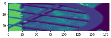
import numpy as np
df = sgm_data.scans['2021-07-29t13-04-30-0600'].entry29['binned']['dataframe']
v = df.filter(regex=("sdd1.*"), axis=1).to_numpy()
sdd1 = np.reshape(v,(len(df.index.levels[0]), len(df.index.levels[1]), v.shape[-1]))

plt.imshow(np.sum(sdd1[:,:,45:55], axis=2).T)

<matplotlib.image.AxesImage at 0x7f852cd3cd00>

png

Utilities¶

Aside from the core use cases, there are some useful utilities for exploring the HDF5 files.

import h5py
from sgmdata.utilities import h5tree, scan_health
from sgmdata import preprocess

scan_health?

preprocess?

preprocess(sample="Test Sample", resolution=0.05)

h5tree?

f = h5py.File("/home/jovyan/data/arthurz/2020-01-07t12-56-39-0600.nxs", 'r')
h5tree(f)

->entry1 <Group> attrs:{NX_class:NXentry,}
|-command <Dataset> type:object shape:() attrs:{}
->data <Group> attrs:{NX_class:NXdata,axes:['yp' 'xp'],signal:sdd3,}
    |-clock <Dataset> type:float32 shape:(3156,) attrs:{units:s,}
    |-emission <Dataset> type:int32 shape:(256,) attrs:{units:eV,}
    |-i0 <Dataset> type:float32 shape:(3156,) attrs:{gain:1 mA/V,units:a.u.,}
    |-pd <Dataset> type:float32 shape:(3156,) attrs:{gain:5 uA/V,units:a.u.,}
    |-sdd1 <Dataset> type:float64 shape:(3156, 256) attrs:{NX_class:NXdetector,}
    |-sdd2 <Dataset> type:float64 shape:(3156, 256) attrs:{NX_class:NXdetector,}
    |-sdd3 <Dataset> type:float64 shape:(3156, 256) attrs:{NX_class:NXdetector,}
    |-sdd4 <Dataset> type:float64 shape:(3156, 256) attrs:{NX_class:NXdetector,}
    |-temp1 <Dataset> type:float32 shape:(3156,) attrs:{NX_class:NX_TEMPERATURE,conversion:T = 5.648
    |-temp2 <Dataset> type:float32 shape:(3156,) attrs:{NX_class:NX_TEMPERATURE,conversion:T = 5.648
    |-tey <Dataset> type:float32 shape:(3156,) attrs:{gain:1 mA/V,units:a.u.,}
    |-wavelength <Dataset> type:float64 shape:(1044,) attrs:{units:nm,}
    |-xeol <Dataset> type:float64 shape:(3156, 1044) attrs:{NX_class:NXdetector,}
    |-xp <Dataset> type:float32 shape:(3156,) attrs:{units:mm,}
    |-yp <Dataset> type:float32 shape:(3156,) attrs:{units:mm,}
|-defintion <Dataset> type:object shape:() attrs:{}
->instrument <Group> attrs:{NX_class:NXinstrument,}
    ->absorbed_beam <Group> attrs:{NX_class:NXdetector,}
    ->fluorescence <Group> attrs:{NX_class:NXfluorescence,}
    ->incoming_beam <Group> attrs:{NX_class:NXdetector,}
    ->luminescence <Group> attrs:{NX_class:NXfluorescence,}
    ->mirror <Group> attrs:{NX_class:NXmirror,}
        |-kbhb_d <Dataset> type:object shape:() attrs:{}
        |-kbhb_u <Dataset> type:object shape:() attrs:{}
        |-kblh <Dataset> type:object shape:() attrs:{}
        |-kblv <Dataset> type:object shape:() attrs:{}
        |-kbvb_d <Dataset> type:object shape:() attrs:{}
        |-kbvb_u <Dataset> type:object shape:() attrs:{}
        |-stripe <Dataset> type:object shape:() attrs:{}
    ->monochromator <Group> attrs:{NX_class:NXmonochromator,}
        |-en <Dataset> type:object shape:() attrs:{units:eV,}
        |-en_err <Dataset> type:int64 shape:() attrs:{units:E/dE,}
        ->exit_slit <Group> attrs:{NX_class:NXslit,}
            |-exit_slit <Dataset> type:float32 shape:() attrs:{units:μm,}
            |-exs <Dataset> type:object shape:() attrs:{units:mm,}
        ->grating <Group> attrs:{NX_class:NXgrating,}
            |-coating_material <Dataset> type:object shape:() attrs:{}
            |-coating_roughness <Dataset> type:int64 shape:() attrs:{units:rms(Å),}
            |-coating_thickness <Dataset> type:int64 shape:() attrs:{units:Å,}
            |-deflection_angle <Dataset> type:int64 shape:() attrs:{units:degrees,}
            |-interior_atmosphere <Dataset> type:object shape:() attrs:{}
            |-period <Dataset> type:object shape:() attrs:{}
            |-sgm <Dataset> type:object shape:() attrs:{units:mm,}
            |-shape <Dataset> type:object shape:() attrs:{}
            |-substrate_material <Dataset> type:object shape:() attrs:{}
    ->source <Group> attrs:{NX_class:NXsource,}
        |-current <Dataset> type:float32 shape:() attrs:{units:mA,}
        |-name <Dataset> type:object shape:() attrs:{}
        |-probe <Dataset> type:object shape:() attrs:{}
        |-sr_energy <Dataset> type:float64 shape:() attrs:{units:GeV,}
        |-top_up <Dataset> type:object shape:() attrs:{}
        |-type <Dataset> type:object shape:() attrs:{}
        |-und_gap <Dataset> type:object shape:() attrs:{units:mm,}
->monitor <Group> attrs:{NX_class:NXmonitor,}
|-proposal <Dataset> type:object shape:() attrs:{}
->sample <Group> attrs:{NX_class:NXsample,}
    |-description <Dataset> type:object shape:() attrs:{}
    |-image <Dataset> type:uint8 shape:(1200, 1600, 3) attrs:{CLASS:IMAGE,IMAGE_SUBCLASS:IMAGE_TRUEC
    |-name <Dataset> type:object shape:() attrs:{}
    ->positioner <Group> attrs:{NX_class:NXpositioner,}
        |-hex_x <Dataset> type:object shape:() attrs:{units:mm,}
        |-hex_y <Dataset> type:object shape:() attrs:{units:mm,}
        |-hex_z <Dataset> type:object shape:() attrs:{units:mm,}
        |-zp <Dataset> type:object shape:() attrs:{units:mm,}
    ->potentiostat <Group> attrs:{NX_class:NXvoltage,}
    ->temperature <Group> attrs:{NX_class:NXtemperature,}
|-start_time <Dataset> type:object shape:() attrs:{}
|-user <Dataset> type:object shape:() attrs:{}

Example Usage¶

Dask Background¶

Searching for Data¶

class SGMQuery(**kwargs):¶

Attributes¶

Loading Data¶

class SGMData(file_paths, **kwargs):¶

arg¶

Keywords¶

Functions¶

Attributes¶

The SGMScan object¶

Plotting Scan Data¶

Interpolating Data¶

Batch interpolation¶

Averaging Data¶

Fitting XRF Spectra¶

Utilities¶

sgm-data

Navigation

Related Topics